Point Cloud Object Classification with Voxel Featurization
Introduction
Cepton's perception team is actively developing a system to classify point cloud objects acquired from their LiDAR sensor. Neural networks are widely known as the state-of-the-art approach to tackle the task of classification, and Cepton LiDAR's high-resolution point cloud can be used with them, although efficient and accurate featurization has to be completed first.
In my internship, I integrated a voxel featurization into their system and tested its capability. In this post, I will go over how point cloud data are featurized as voxel data and how the neural network architecture is tailored for voxel featurization. In the end, I briefly report that my voxel featurization showed high efficiency and accuracy for the object classification task.
Featurization
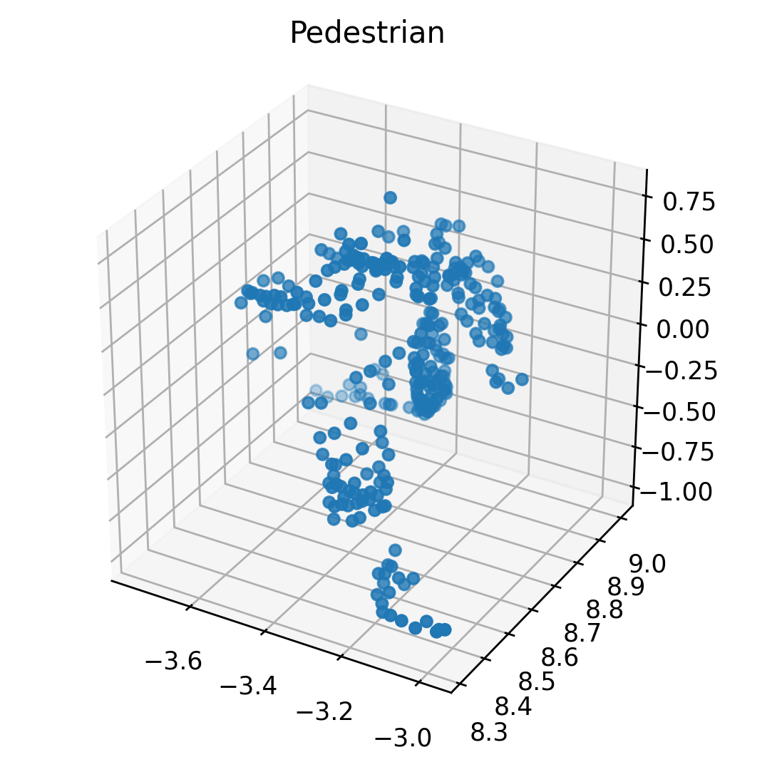
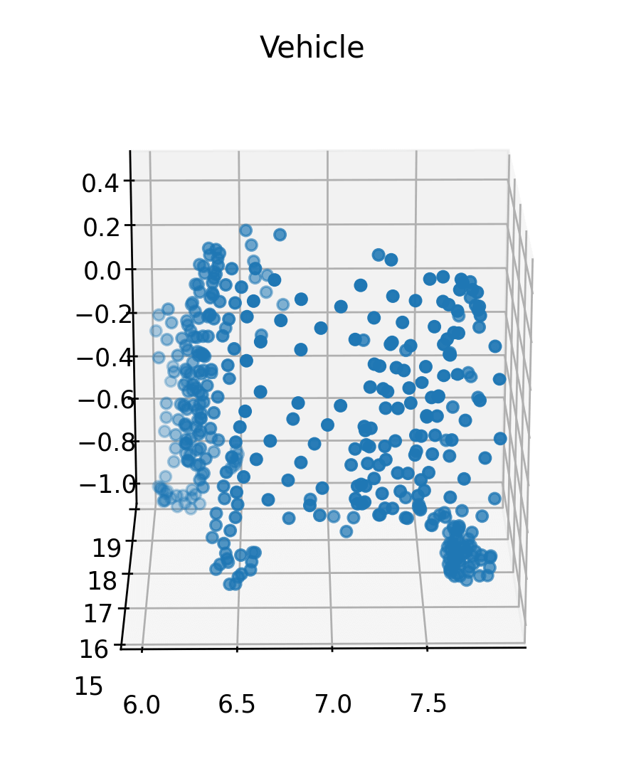
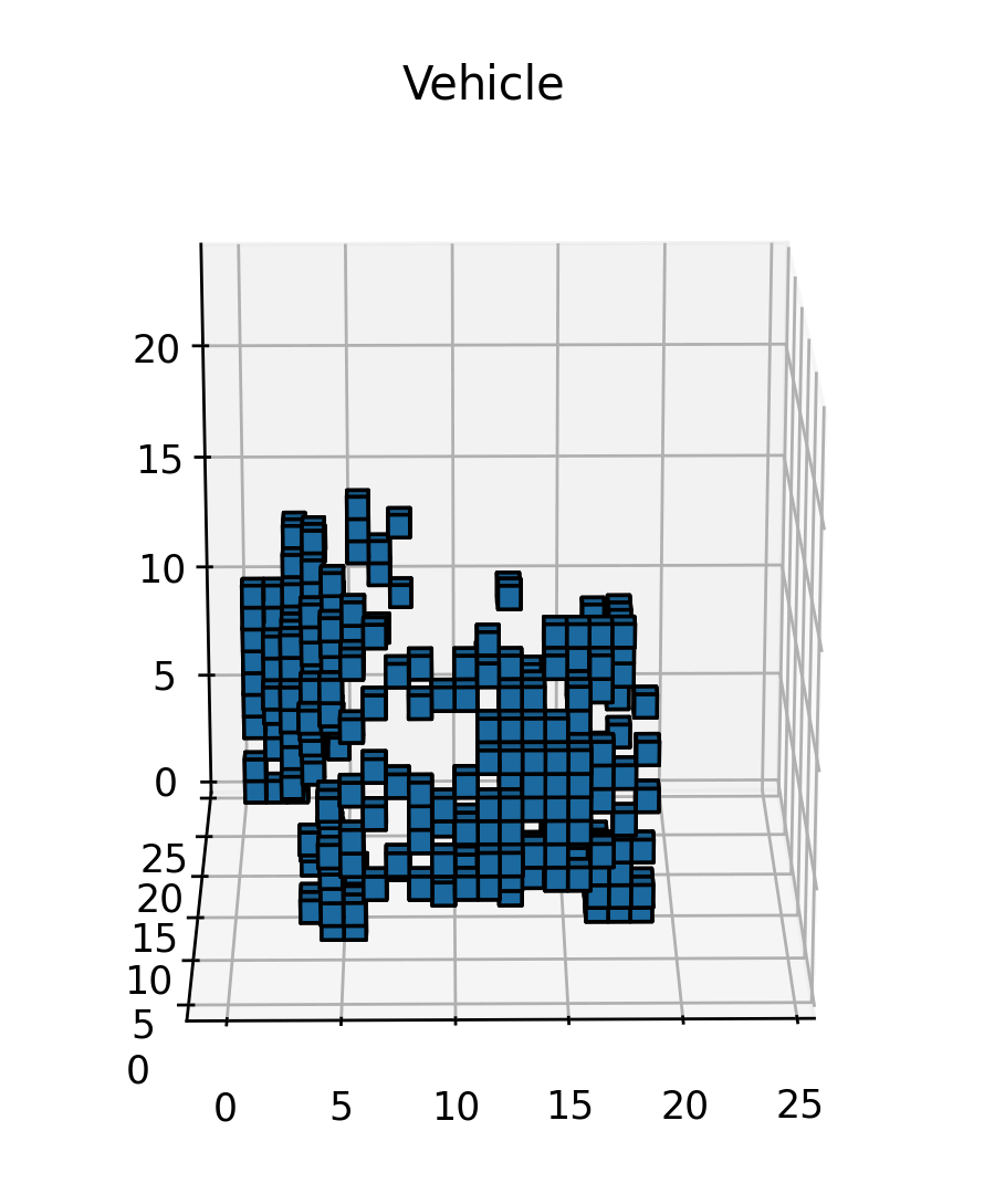
Data collected from our LiDAR sensors takes the shape of a point cloud, with each point having position information in the form of coordinates. However, these unstructured points can’t easily be used in a neural network, so they must be converted to some structured form first, i.e. the input data has to be featurized. There are many different ways of doing this, with the one I chose being a 3D voxel grid.
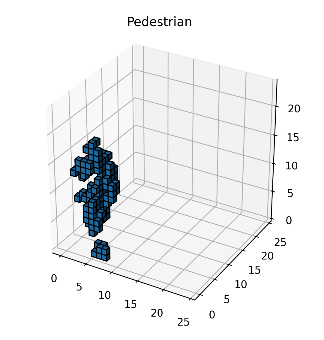
I start with normalizing the points to the origin. I compute the minimum value for each dimension across the entire point cloud and then translate all points by subtracting these minimum values, aligning the point cloud with the origin. I use cubical voxels of size , each of which is set to be 1.0 if it contains a point in it, otherwise 0.0. I set the number of voxels as (2.4m each), to well capture both pedestrians and vehicles.
Once this was done for all of the points, it resulted in a collection of voxels that represented the point cloud. Finally, I converted the grid into a tensor, which could then be fed into a neural network, which I will explain next.
import numpy as np
import torch

def featurize(point_cloud):
  # Find min and normalize
  minX = min(data, key=lambda x: x[0])[0]
  minY = min(data, key=lambda x: x[1])[1]
  minZ = min(data, key=lambda x: x[2])[2]
  data = [(x - minX, y - minY, z - minZ) for [x, y, z] in data]
  width = 0.1
  # Create grid and fill with zeros
  grid_size = 24
  voxelGrid = np.zeros((min_grid_size, min_grid_size, min_grid_size), dtype=float)
  # Fill in grid
  for [x, y, z] in data:
      indexX, indexY, indexZ = int(x / width), int(y / width), int(z / width)
      indexX = min(indexX, grid_size - 1)
      indexY = min(indexY, grid_size - 1)
      indexZ = min(indexZ, grid_size - 1)
      voxelGrid[indexX, indexY, indexZ] = 1

  # Convert a NumPy array to a Tensor
  voxelTensor = torch.from_numpy(voxelGrid)
  return voxelTensor
Neural Network Architecture
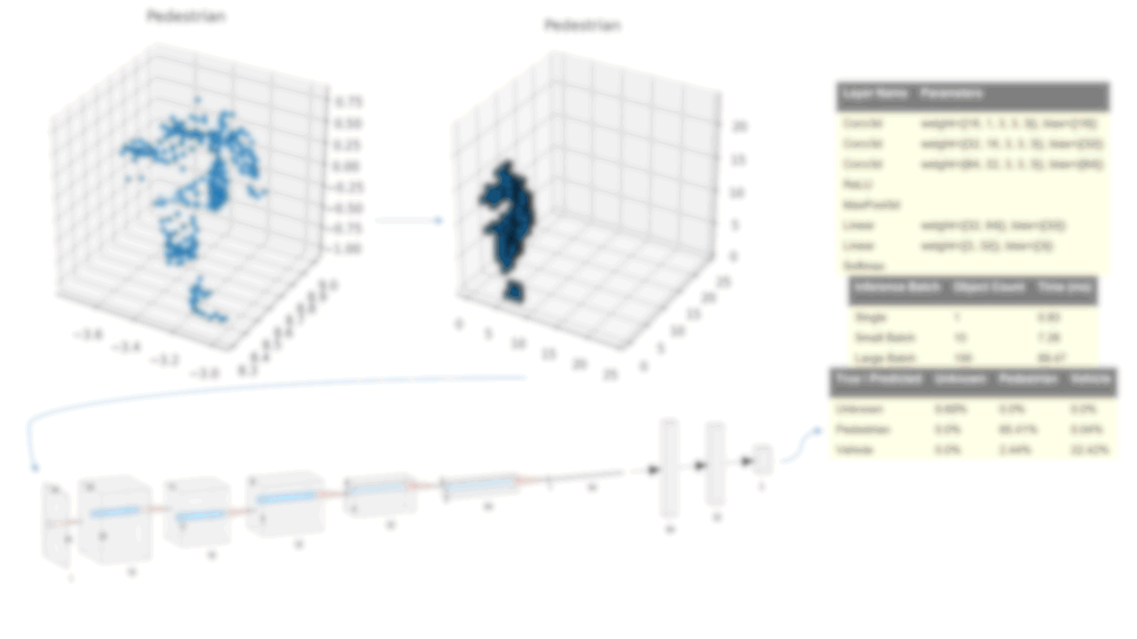
After featurizing the point cloud data, the next step is to feed them to a convolutional neural network (CNN) to build a classifier. The reason that this has to take place after featurization is that the point cloud data lacks a clear structure and features to learn from. However, featurizing the points as voxels gives CNN a structure to work with, which greatly benefits the learning process.
This type of neural network consists of multiple convolutional layers with max pooling and activation functions, followed by fully connected layers and a final output layer. For my classifier, which I implemented in PyTorch Lightning, I pretty much followed the standard structure : I had three convolutional layers, each followed by a max pool and ReLU, then two fully connected layers using a linear transformation, with the first one followed by ReLU, and finally a softmax and output layer. Because the data was in three dimensions, I used the three-dimensional versions of the convolution and max pool functions.
Throughout this process, the dimensions go from while the number of filters goes from and the kernel size stayed constant at . See the figure below for the details.
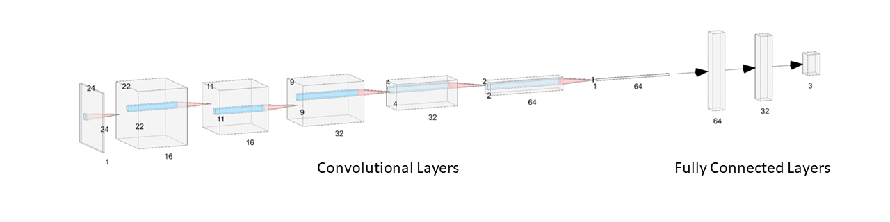
Note: this figure isn't completely accurate because the visualization tool doesn't support three-dimensional convolutions, but it's a fair approximation.
Results and Revisions
The classifier achieved good accuracy, with > 99% on pedestrians and > 90% on vehicles. The speed was also reasonably fast, although not the fastest out of all the classifiers available.
| True/Predicted | Unknown | Pedestrian | Vehicle |
|---|---|---|---|
| Unknown | 9.69% | 0.0% | 0.0% |
| Pedestrian | 0.0% | 65.39% | 0.06% |
| Vehicle | 0.0% | 2.71% | 22.15% |
| Inference Batch | Object Count | Time (ms) |
|---|---|---|
| Single | 1 | 0.83 |
| Small Batch | 10 | 7.28 |
| Large Batch | 100 | 89.47 |
Further Extension
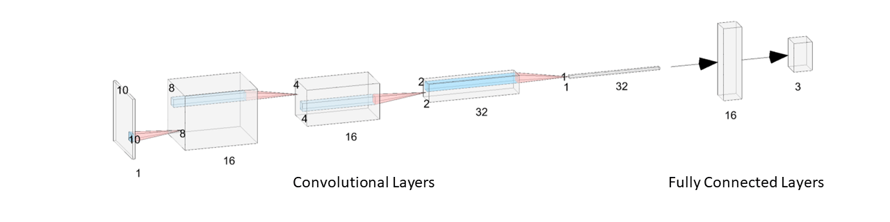
As an extension, I experimented with dropping the final convolutional layer and its associated max pool and ReLU, while reducing the initial dimensions of the grid to a . This resulted in the number of filters topping out at , and the dimensions going from . These changes were effective, with the classifier's speed improving significantly ( faster) while accuracy remained the same.
| Inference Batch | Object Count | Time (ms) |
|---|---|---|
| Single | 1 | 0.26 |
| Small Batch | 10 | 0.81 |
| Large Batch | 100 | 2.59 |
Conclusion
In this post, I went over the voxel featurization and the CNN architectures to featurize and classify point cloud data. The classifier I implemented was able to achieve high accuracy and speed. In the future, the accuracy could be improved with greater amounts of training data, and the speed could likely be increased with further refinements to the neural net architecture.