Lidar Camera Calibration Pipeline

Cover photo courtesy Andrew Lauer.

Introduction

Lidar camera calibration is the process of estimating the pose of a camera relative to a lidar. To achieve this, one must find corresponding points in space between the two perspectives. The most straightforward way to do this is by locating an object that appears in both the lidar and camera views.

As with any model, the more data points available, the more accurate the resulting calibration will be. There are two simple methods of achieving this:

(a) Detect multiple objects in different locations simultaneously

(b) Track one object that moves to different positions over time

This blog explains the second approach, and the challenges/methodology associated with each step along the way. 

Part 1: Defining Prerequisites

Before beginning calibration, one must first consider the form and collection of the data used. The goal is to have many matching lidar and camera frames of the same object in different locations. The simplest solution? A lidar and a camera recording of the same moving object.

Lidar recording is simple; Cepton already has a well-defined architecture for the collection and handling of lidar data.

Camera recording, on the other hand, is unfortunately less trivial. Different camera manufacturers have different SDKs, and most of them don't play well with Rust—the language of choice for Cepton software. Luckily, the camera manufacturer we chose to support, Basler, provided a C++ library for which someone wrote a Rust linking wrapper for: Pylon CXX.

But just having two recordings isn't enough; The lidar and camera data must be synchronized. Since the object is moving, we need lidar and camera frames of the same timestamp to get corresponding points.

Thus, we require three things to start calibration:

(a) A lidar recording

(b) A camera recording

(c) Some way of syncing the lidar and camera

Ideally, for ease of handling and future-proofing the data, we can have one piece of data/software that collects and handles all three pieces.

Luckily, such a system already exists:

Part 2: The CR (Cepton Record) Format

The Cepton Record format was designed for this exact purpose: To collect multiple streams of data and combine them into one .cr file. It supports streams of lidar frames, images, and IMU data (although IMU is an orientation sensor, and isn't used in this project).

Perfect right? But there's one catch: the CR format supports images, not video. This means that in order to utilize the existing CR format framework, we would need to write every single image for every camera frame to the resulting file.

Optimally, for machine learning purposes, we want to support video frames that are both frequent and high resolution. But both of these factors make it extremely space-intensive to write every single camera image.

Example: Why Writing Individual Frames Isn't Feasible

Let's start with some back-of-the-envelope math.

With the Basler acA2440-20gm, we can get up to 2448 x 2048 frames at 23 fps.

At no image compression (writing .bmp files), a .cr of a ~15-second recording would be estimated to look something like this:

${15 sec} \times {23 frames/sec} \times {{(2448 \times 2048)} pixels/frame} \times {24 bits/pixel} = {{41511813120} bits} = {{5188976640} bytes} \approx {{5189} MB}$

Yikes. 5 gigabytes for a 15-second recording. Not to mention that this is an underestimate; We're not even taking into account the size of the bitmap header.

We can try compressing the image to different formats, like .jpg. Assuming an aggressive (and unrealistic) 50 to 1 compression ratio, we get:

${{5189} MB} \times \frac{1}{50} \approx {{104} MB}$

Definitely better. But compressing images along with recording takes time, and is difficult to make fast enough to match the frames per second. This means we end up with a backlog that grows the longer we record (eating up memory and performance).

In comparison, an .mp4 is usually magnitudes smaller than the JPGs. This is because video formats (like .mp4) get most of their space savings due to their ability to encode differences between adjacent frames rather than the entire frame itself.

To illustrate this:

A Real Example

Here is a 30-second video of a moving chessboard:

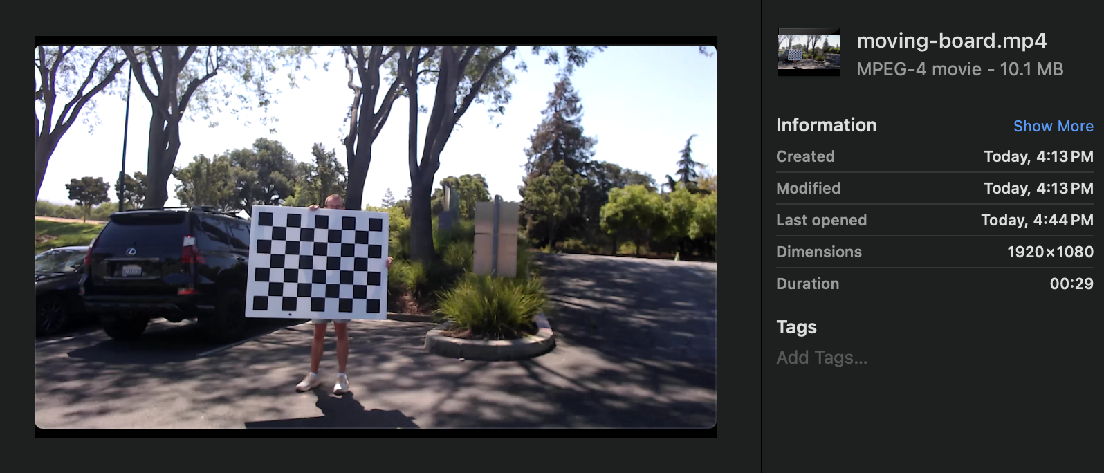
It's 10.1 MB.

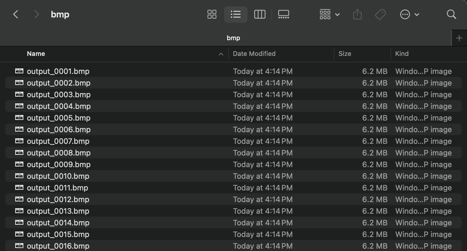
Using ffmpeg, the video is split into separate images, one for every frame. This is done three times, with the images being in the formats .bmp, .png, and .jpg. Each time, the resulting images are put in a folder named bmp, png, and jpg, respectively.

Here is the BMP folder for reference:

Now, here are the sizes of the resulting splits:

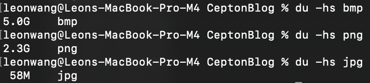
Surprisingly, JPG compression is much better than expected. However, it is still 6x larger than the MP4.

This example makes the limitations of frame-by-frame storage clear.

The Solution: Use Videos

As the header says, the solution is to just use videos. They are better in both space efficiency and accessibility.

But this introduces a new challenge: How do we integrate videos into the CR format?

Simply writing the entire .mp4 into the .cr is both clunky and hard to validate. Not to mention, we'll need to write a custom .mp4 parser if we want to efficiently read the video(s) from and to part(s) of a .cr file—far outside the scope of this task.

Let's take a step back. Consider the third piece of data, the offset. Notice, one will never have an offset without a corresponding video.

What if each offset record also came with a relative file path to a .mp4 file written outside the .cr?

Unfortunately, this solution means compromising on the original goal of not having multiple files. But, it comes with multiple upsides as well:

(a) Easier parsing

(b) Easier validation (you can just open up the .mp4 manually)

(c) Faster development time

As such, this is the solution we chose.

Part 3: Recording Data

The Cepton Record format is accompanied by a corresponding Rust tool: The Cepton Record Recorder. It already supports recording with lidar and IMU, and modifying it to support a camera as well is not too difficult with the existence of the previously mentioned Pylon CXX.

However, we encountered several challenges.

Capturing Video from Camera Frames

The first issue was that Pylon provides access to each frame's image when recording; It doesn't support native video recording. Thankfully, tools ffmpeg which turn images into video already exist. Using it through the ffmpeg-sidecar crate, we can write a camera's separate image frames into one aggregate .mp4 at a speed which keeps up with the frame rate.

Synchronizing Lidar and Camera

The second issue was related to time syncing. Since we only record the offset between the beginning of the video and the lidar, we need to accurately determine the time between a frame and the start of the recording.

This is trivial for the lidar: Every frame has its own timestamp.

The video, however, is trickier. While videos have a constant frame rate, the actual delivery of the frames from the camera is inconsistent: Every once in a while, there will be a frame that is "dropped" (not received). Thus, we need a way to "fill" in the gaps.

The solution: Assume the fetching of images is non-deterministic. At every timestamp where we expect a frame, we write the most recent successfully fetched frame.

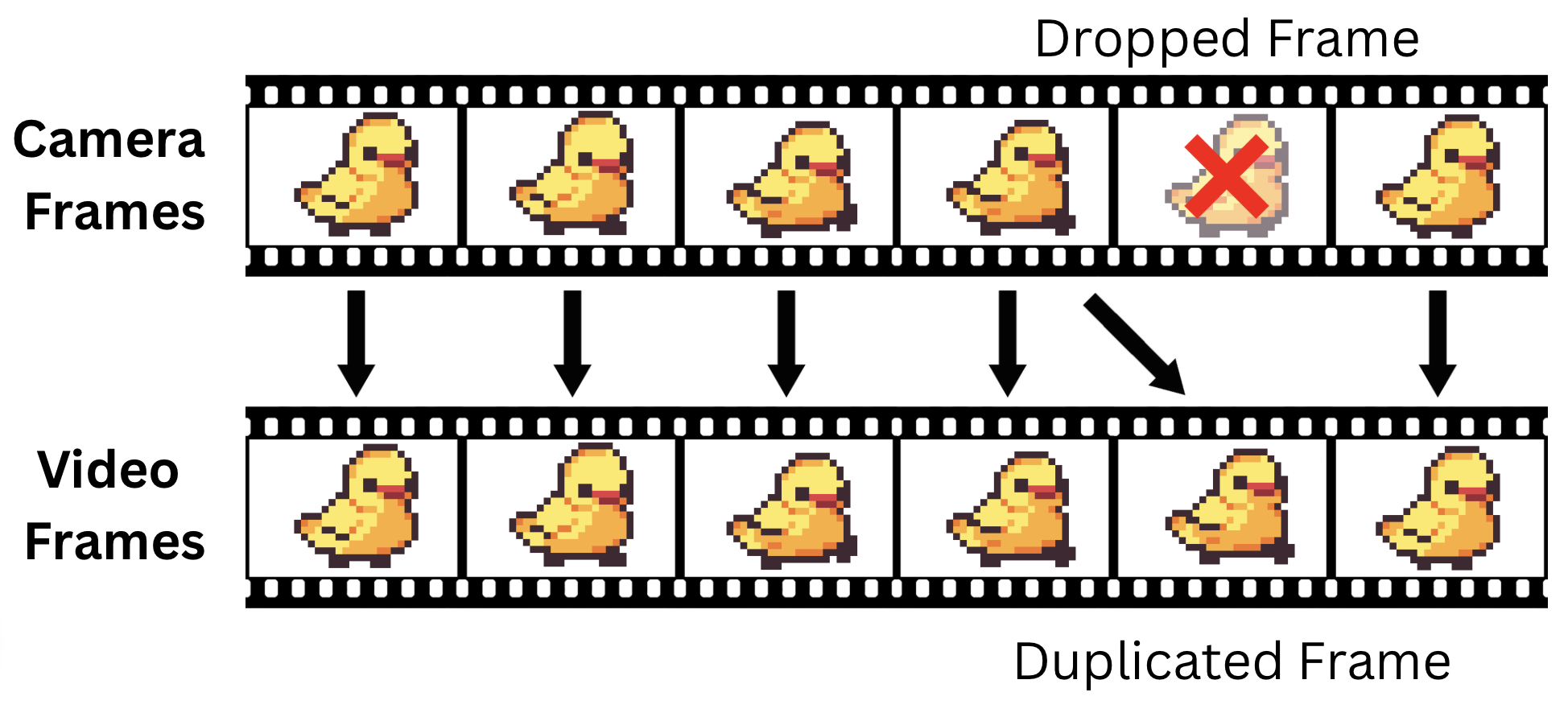
This method handles dropped frames rather gracefully. While it does introduce small timing inaccuracies, it is mostly negligible for our purposes; The calibration objects should not be moving fast enough for that to matter.

Part 4: Lidar Camera Calibration

With both synchronized recordings, we can finally feed the data into a pipeline that takes corresponding frames, finds a common object, and then estimates the pose of the camera.

While the input portion of the pipeline (reading in recordings and matching the frames by timestamps) is still in progress, a basic version of the calibration pipeline has been implemented.

Andrew Lauer has both implemented and written an excellent explanation of the calibration process in repository ceptontech/lidar_camera_calibration, which he has graciously given permission for me to share:

---

Lidar camera calibration is the process of finding the projection matrix $P$, a 3 by 4 matrix that projects a 3d world point $X_i$ to a 2d image point $x_i$ in a camera. The projection matrix also encodes useful information about the position of the camera and the camera itself. World and image points are expressed in homogeneous coordinates.

The process starts by matching 2d points in the image to corresponding 3d points in the point cloud. This can be done using any standard method using chessboards, fiducial markers, or feature detection. However, since the point cloud contains 3d information, the points must be projected to a plane, similar to a camera. The following equation shows how the projection matrix relates world points to image points.

$PX_i = x_i$

$\begin{bmatrix}p_{11} & p_{12} & p_{13} & p_{14} \\\ p_{21} & p_{22} & p_{23} & p_{24} \\\ p_{31} & p_{32} & p_{33} & p_{34}\end{bmatrix}\begin{bmatrix}X \\\ Y \\\ Z \\\ 1\end{bmatrix}=\begin{bmatrix}u\\\ v\\\ 1 \end{bmatrix}$

This can be rewritten to express the image point as follows:

$x_i = \begin{bmatrix}\frac{p_1^TX_i}{p_3^TX_i}\\\ \frac{p_2^TX_i}{p_3^TX_i}\\\ 1\end{bmatrix}=\begin{bmatrix}u\\\ v\\\ 1\end{bmatrix}$

And then for each world/image pair:

$p_1^TX_i-u_ip_3^TX_i=0$

$p_2^TX_i-v_ip_3^TX_i=0$

Doing this for all pairs of world and image points, we can construct the matrix A as follows:

$A \vec{p} = \begin{bmatrix} X_1^T & \vec{0} & -X_1^Tu_1 \\\ \vec{0} & X_1^T & -X_1^Tv_1 \\\ \vdots & \vdots & \vdots \\\ X_n^T & \vec{0} & -X_n^Tu_n \\\ \vec{0} & X_n^T & -X_n^Tv_n \end{bmatrix}_{\text{2nx12}} \begin{bmatrix} \vec{p_1} \\\ \vec{p_2} \\\ \vec{p_3} \end{bmatrix} = \begin{bmatrix} 0 \\\ 0 \\\ \vdots \\\ 0 \\\ 0 \end{bmatrix}$

Applying SVD to $A$ gives us an initial guess for $p$ that minimizes the $Ap$ product. I.e. $p\in Null(A)$.

This guess can be improved by applying the Levenberg-Marquardt non-linear iterative least squares method. The cost function for the LM optimization is the distance between the ground truth image points and the 3d points projected into the image plane.

Once a good estimation for $P$ has been found, the camera intrinsics, rotation, and translation matrices can be found by decomposing the projection matrix with RQ decomposition. This is a straightforward decomposition, since the projection matrix is defined by:

$P = K[R|t]$

Summary

To estimate the pose of the camera relative to the lidar frame, we must find the projection matrix $P$ which maps lidar points to the image plane. This can be done in the following steps:

(a) Match 3D and 2D point pairs

(b) Create a linear system with the point data

(c) Find an initial guess for the solution with SVD

(c) Use Levenberg-Marquardt to refine the solution

(d) Decompose the result to find the camera intrinsics, rotation, and translation matrices

Part 5: Future Usage

With the entire pipeline implemented, we open ourselves up many possibilities such as:

(a) Depth camera: By projecting all the lidar points into the camera frame, we can effectively simulate a depth camera

(b) Validation and debugging: With synchronized video and lidar data, future lidar recordings will be easier to visually inspect and debug

(c) Lidar-camera system integration: Any system with both lidar and camera will benefit from having an accurate calibration system

However, the most useful application is as follows:

Utilization of Imagery CV

First, it is important to understand that computer vision models for camera are much more sophisticated than the corresponding models for lidar. This is simply by virtue of the focus of the computer vision industry being primarily on imagery.

By having a way to convert between imagery and lidar, we open ourselves up to the possibility of using computer vision models for imagery to help develop corresponding tools for lidar.

Unfortunately, while the projection matrix provides a way to convert from camera to lidar data, the reverse isn't as simple. Notice that camera data is in two dimensions, and lidar data is in three. This means a degree of information is lost when converting from lidar to camera. And as such, when we convert from camera back to lidar, one degree of freedom is introduced. Each camera point will correspond not to a point, but a line in the lidar.

Despite this ambiguity, this data is still valuable—as a constraint for data expected from our lidar computer vision models.

Consider a computer vision model run on a video of a parking lot. With the objects detected in the frame we can:

(a) Cross-reference it with output generated by a lidar model run on the corresponding lidar data, providing weak supervision/validation

(b) Quickly generate labels for lidar data to train future models on

Both of which will help streamline the process of training future lidar computer vision models.

Conclusion

The lidar camera calibration pipeline unifies two separate perspectives, paving the way for improved data handling/collection, easier validation/debugging, and also enhanced sensor fusion.

More importantly, by utilizing the maturity of current image computer vision models, we hope to be able to accelerate the training and accuracy of lidar-based models.

Lidar camera calibration is not just about calibration—it's about combining the strengths of lidar and camera models to accelerate computer perception as a whole.