Real-Time PCAP Data Overlay Over Synthetic Geometries

Introduction
The successful development of LiDAR (Light Detection and Ranging) systems is expedited by simulations, i.e. to test in extreme scenarios and reduce costs compared to extensive real-world testing. Though, Cepton's internal real-time simulator, while substantial in simulation cases and objects, cannot always replicate real-world environments due to the requirements of dense, accurate mesh maps that are difficult to replicate procedurally. Henceforth, we add new logic to the simulator that lets us load in data recorded from a live sensor to overlay the simulated geometries for more accurate simulation.
Background Profile Generator
The first step in enabling real-world data overlay involves creating a background profile generator that captures the static environment from PCAP recordings. This component processes LiDAR frames to build a depth map representing the furthest observable surfaces. Our approach was to process the number of frames and update an internal 2D buffer and write to a bitmap file to create the foundational depth data needed for AR simulation overlays.
For example, something like this:
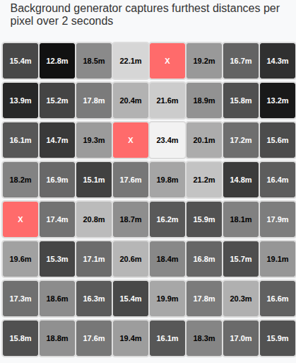
depth_map[ez][ex] = distance_mm; //store the max distance per pixel (e.g. depth_map[0][0] = 15420.5mm, 15.42 meters)
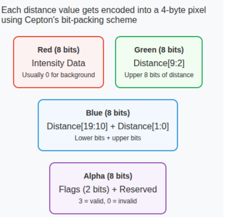
You can store a lot of information in a 2d bitmap image! Each distance gets packed into a 32-bit RGBA pixel using Cepton's SDK bit-packing scheme:
Encode pixels by converting depth map to sdk pixel format:
for ez in 0..self.image_height as usize {
    for ex in 0..self.image_width as usize {
        let distance_mm = self.depth_map[ez][ex];

        if distance_mm > 0.0 {
            // it is a valid pixel, so create a proper Pixel struct and encode it correctly
            let mut pixel = Pixel::default();

            // set distance (uses 20 bits: 10 bits in green + 10 bits in blue)
            let distance_u32 = (distance_mm as u32).min(0xFFFFF);
            pixel.set_distance(distance_u32);

            // set flags (uses 2 bits in alpha channel)
            pixel.set_flags(3); // Valid pixel flag

            // convert pixel to bytes
            let pixel_bytes = pixel.as_bytes();
            image_data.extend_from_slice(pixel_bytes);
        } else {
            // otherwise this is invalid
            let mut invalid_pixel = Pixel::default();
            invalid_pixel.set_distance(0);
            invalid_pixel.set_flags(0);
            invalid_pixel.set_intensity(0);

            let pixel_bytes = invalid_pixel.as_bytes();
            image_data.extend_from_slice(pixel_bytes);
        }
    }

    // row padding
    image_data.extend(std::iter::repeat_n(0, padding_per_row as usize));
}
We output two complementary outputs:
(1) SDK-Compatible Depth Image ready to load into the simulator.
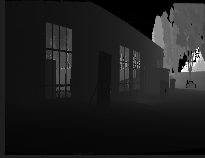
(2) A standard grayscale bitmap for visual sanity checking, where the pixel intensity represents distance.
AR Background Integration Pipeline
From a software engineering perspective, one must consider how to seamlessly integrate this new overlay pipeline into complex preexisting rendering engine architecture.
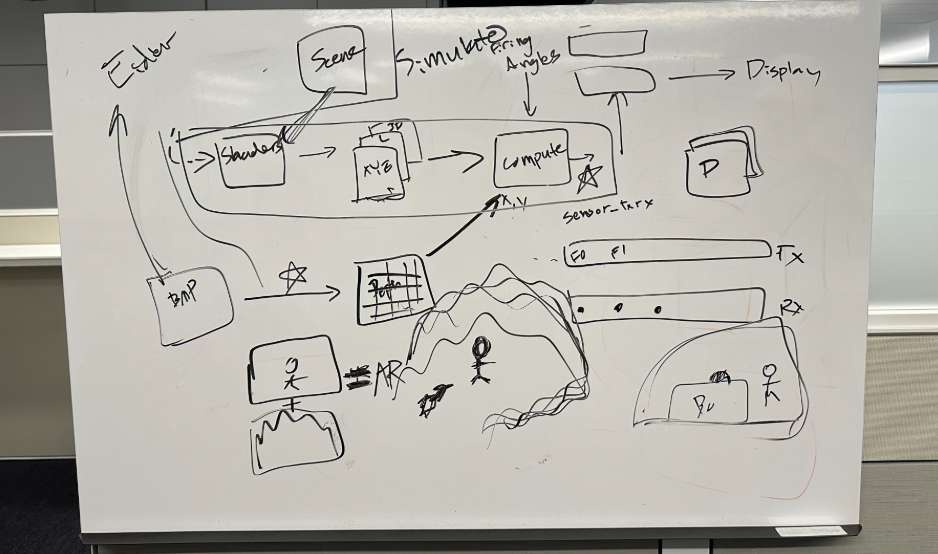
While Cepton's simulation already features a robust multi target rasterization system for synthetic objects, we needed to figure out how to add a parallel AR Pipeline that operates alongside the existing render targets. This addition would preserve the original simulation capabilieis while enabling the new ability to blend with recorded LiDAR data.
We introduce a new dedicated texture pipeline specifically for background profile data. Our design decision here was to use the R32Float format to store millimeter-precision distance values directly, rather than RGBA position textures which store 3D coordinates.
//  new pipeline for overlay-specific texture creation
let ar_texture = Texture::create_ar_background_profile_texture(device, &dims, "ar texture");

pub fn create_ar_background_profile_texture(
    device: &Device,
    size: &[u32; 2],
    label: &str,
) -> Self {
    let texture = device.create_texture(&TextureDescriptor {
        label: Some(label),
        size: Extent3d {
            width: size[0],
            height: size[1],
            depth_or_array_layers: 1,
        },
        format: TextureFormat::R32Float,  // single-channel distance data
        usage: TextureUsages::TEXTURE_BINDING | TextureUsages::COPY_DST,
        // ... other properties
    });
}
We implement the AR pipeline system that does full BMP parsing and uploading,operating independently of the rest of the engine rasterization:
impl ARSimExt {
    fn new(
        device: &Device,
        queue: &Queue,
        layout: &BindGroupLayout,
        texture: Texture,
        bmp_path: String,
    ) -> Self {
        // ...logic to parse and extract encoded distnace values from bitmap
          //...logic to load in file
          let bmp_image = Self::parse_bmp_manually(&bmp_bytes)

        // upload this to the GPU Texture
        Self::write_bmp_to_texture(queue, &texture, &bmp_image);

        // create dedicated bind group for AR pipeline
        let bind_group = device.create_bind_group(&wgpu::BindGroupDescriptor {
            label: Some("ar_sim_bind_group"),
            layout,
            entries: &[BindGroupEntry {
                binding: 0,
                resource: wgpu::BindingResource::TextureView(&texture.view),
            }],
        });

        ARSimExt { bmp_image, bind_group, background_profile_texture: texture }
    }
}
We then do a GPU texture upload and a parallel pipeline integration. Once again, the AR background profile operates as a parallel data source alongside the traditional rasterization pipeline:
// traditional rasterization still occurs normally
let mut render_pass_1 = encoder.begin_render_pass(&wgpu::RenderPassDescriptor {
    color_attachments: &[
        Some(position_texture),     // Synthetic object positions
        Some(reflectivity_texture), // Synthetic material properties
        Some(object_id_texture),    // Synthetic object IDs
        Some(label_texture),        // Synthetic semantic labels
    ],
    // ... render synthetic geometry
});
// (consumed later in compute shader, not during rasterization)
We then create a separate bind group layout for this overlay to integrate with the existing compute pipeline.
Overall, this integration adds minimal overhead to the existing rasterization -- minimal GPU memory added (a single R32Float texture would be ~16 MB for 2048x2048 resolution), minimal impact to rasterization performance because we preload the data.
The key insight here is that the AR background integration operates as a data augmentation layer rather than a rendering modification. The existing multi-target rasterization continues unchanged, while the AR system provides an additional data source that gets blended in the subsequent compute shader stage. This design preserves all existing simulation capabilities while enabling seamless real-world data integration.
Background Integration Compute Shader
The heart of our overlay system lies in a custom WGSL compute shaders that blends real-world data with synthetic geometry. This shader processes each LiDAR ray individually and makes per-pixel decisions about whether to use simulated objects or recorded background surfaces.
The compute shader receices data through distinct bind groups, each serving a different purpose. We integrate a bind group for AR simulation:
// Group 0: TX/RX Buffers
// read write buffers here

// Group 1: Rasterization Outputs
// position, reflectivity, object_id, label textures

// Group 2: AR Background Profile
@group(2) @binding(0) var ar_sim_buffer: texture_2d<f32>;

// Group 4: Runtime Configuration
@group(4) @binding(0) var<uniform> ar_config: ARSimConfig;
We optimize performance with 256 threads per workgroup for optimal GPU utilization.
We then utilize compute threads to process a single LiDAR "fire" by calculating the ray direction from encoder coordinates. We then turn the angles into a unit vector pointing exactly where the LiDAR beame is firing. Afterwards, our shader implements a decision tree for each ray:
// Step 1: sample the synthetic geometry
let point_position = textureLoad(position_texture, pixel, 0);
let sim_distance = length(point_position.xyz);

// Step 2: Check if our AR option is enabled!
if (ar_config.enabled != 0u) {
    // Step 3: Map encoder coords to AR texture coordinates
    let ar_x = u32(norm_x * f32(ar_dims.x - 1u));
    let ar_y = u32(norm_z * f32(ar_dims.y - 1u));

    // Step 4: sample the background texture
    let background_distance_mm = textureLoad(ar_sim_buffer, ar_pixel, 0).r;

    if background_distance_mm > 100.0 && background_distance_mm < 200000.0 {
        let background_distance_m = background_distance_mm / 1000.0;

        // Step 5: choose the closest surface (synthetic vs background)
        if sim_distance > 0.0 {
            // Both surfaces available always use background for consistent environment
            output_position = transform_to_wgpu_coords(background_distance_m);
            output_object_id = 999999u;  // Background marker
            output_label = 100u;         // Background label
        } else {
            // Only background available
            output_position = transform_to_wgpu_coords(background_distance_m);
            output_object_id = 888888u;  // Background-only marker
            output_label = 99u;          // Background-only label
        }
    }
    // If background invalid, fall back to synthetic geometry
}
Point Cloud Generation
The final stage of AR Pipeline transforms the GPU-processed ray data into a unifed point cloud to finally combine this background data with synthetic objects. We must move the data from GPU to CPU, and apply coordinate transforms.
Each point undergoes validation to track whether it came from synthetic geometry or background data. Then, we must apply the correct coordinate transforms to convert points from LIDAR's local frame to world coordinates.
Our pipeline involves three different coordinate systems:
(1) Cepton LiDAR coordinates: x=right, y=forward, z=up, which matches the physical sensor orientation
(2) WGPU rendering coordinates: x=right, y=up, z=forward, which is standard graphics convention
(3) World coordinates: the final output space for perception algorithms
For PCAP background data, we try to preserve the real-world spatial relationships while only applying minimal transformations needed to account for the sensor's physical mounting. Hence, we use a "ground-only" transformation that applies only height and pitch--the sensor's mounting height above ground plane and the sensor's tilt angle, respectively.
The complete transformation matrix is constructed as:
Where each component is:
T_coord (Coordinate System Transform):
┌  1   0   0  0 ┐
│  0   0  -1  0 │
│  0   1   0  0 │
└  0   0   0  1 ┘
T_height (Height Translation):
┌  1   0   0   0  ┐
│  0   1   0   h  │
│  0   0   1   0  │
└  0   0   0   1  ┘
Where h = sensor mounting height:
R_pitch (Pitch rotation around Z):
┌ cos(θ) -sin(θ)  0  0 ┐
│ sin(θ)  cos(θ)  0  0 │
│   0       0     1  0 │
└   0       0     0  1 ┘
where θ = pitch angle
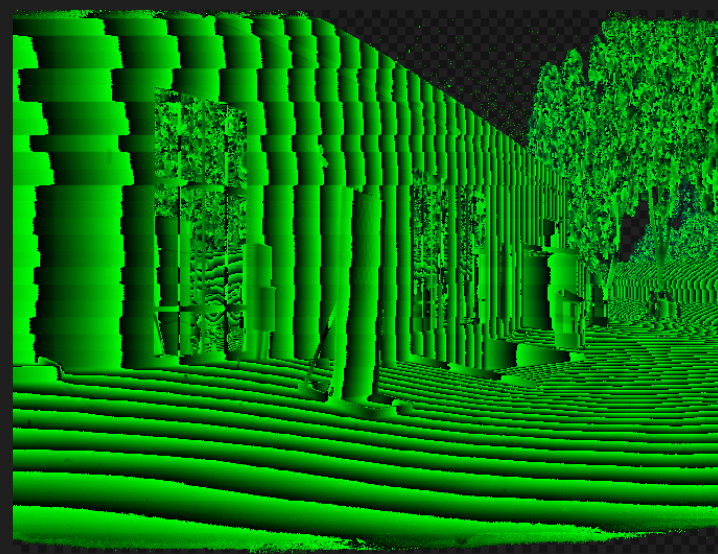
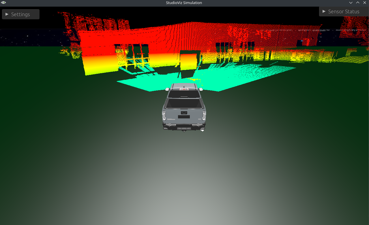
This approach ensures that real-world geometry (buildings, roads, trees), maintains its correct spatial relationships, the sensor appears to be mounted at correct height and angle, and synethetic objects added to the scene align properly with the background. This is an example of what an AR overlay looks like at this point:

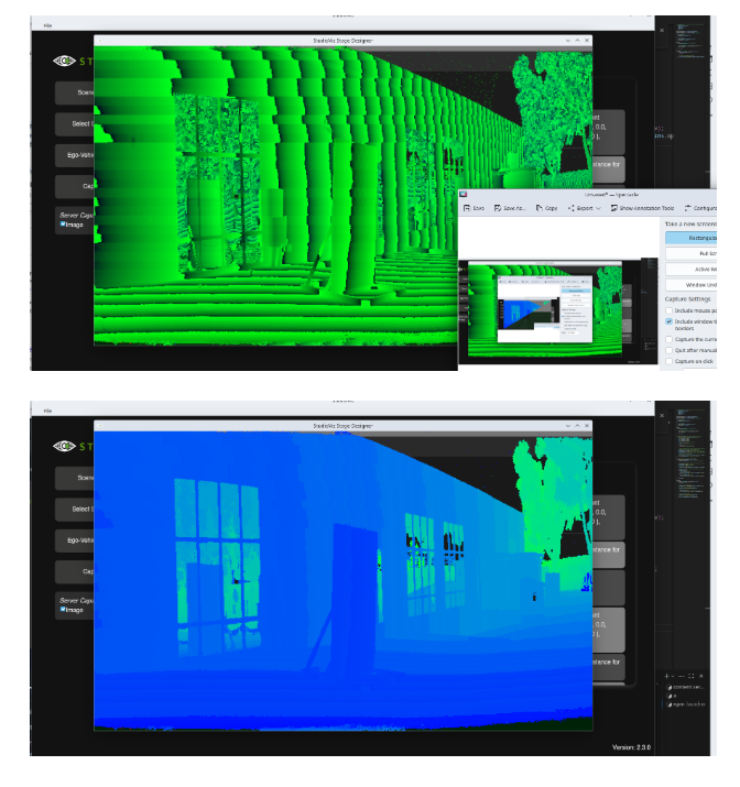
Scene Editor Integration
We apply similar logic to the simulator's scene editor--the pipeline in the simulator that sets spatial properties of each simulated geometry. We add this 3d overlay just so that we can see the 3d points in the scene editor such that we can place objects around it.
Conclusion
With this pipeline implemented, we create more accurate simulations and data that we hope safely accelerates LiDAR development.
Additionally, given the maturity of current computer vision models, we hope this improved data expedites both the training efficiency and accuracy of LiDAR-based models.
References
Kong, F., Liu, X., Tang, B., Lin, J., Ren, Y., Cai, Y., Zhu, F., Chen, N., & Zhang, F. (2023). MARSIM: A light-weight point-realistic simulator for LiDAR-based UAVs. IEEE Robotics and Automation Letters, 8(5), 2626–2633. https://doi.org/10.1109/LRA.2023.3252599